This work was done towards for Stanford University’s CS 221: Artificial Intelligence class project. It was co-authored jointly by Pulkit Agrawal, Maulik Kamdar, Flavia Grey.
You can download this report in PDF Format here (CS221Report)
Introduction
Building energy consumption accounts for close to 50% of the electricity usage in the United States. Building energy simulation models have become an industry standard to help in the decision making process to improve building design in order to reduce consumption, but there is a known discrepancy between these models and actual building energy performance once completed. This is due to their accuracy being compromised by approximations, assumptions and simplifications made in the model. In particular, internal loads are a critical determinant of building performance and their simulation is the most lacking, partly due to simulated occupancy – which accounts for most of a building’s internal loads – being considered discrete, deterministic and unchanging in hour-long periods of time. Previous work has focused mostly on the determination of building occupancy exclusively in terms of presence – whether people are in the space or not – to regulate heating, ventilation and air conditioning systems (HVAC) accordingly. We propose that the type of task the activity level of the occupants also impacts the building’s performance, and viceversa – the building’s performance impacts occupant state. For this purpose, we will analyze building sensor data along wearable sensor data on the occupant measured simultaneously in a controlled environment in order to classify occupant activity levels and determine the distinct impacts on the space occupied by the user.
Related Work
There has been some research in the application of Artificial Intelligence methods to adapt environmental conditions according to user preferences. This branch of AI, called Ambient Intelligence, generally exploits the information about the environment state through cheap and unobtrusive sensors for continuous monitoring. A HVAC control strategy based on occupancy prediction and real time occupancy monitoring via a sensor network of cameras was proposed by Erickson et al [1]. A technique to determine the occupancy and indoor environment quality (IEQ) in buildings by enhancing physical measurements from a distributed sensor network with a statistical estimation method was proposed by Han et al [2]. They used passive infra-red (PIR) sensors, Carbon Dioxide (CO2) concentration sensors, and relative humidity (RH) sensors, and modelled the occupancy pattern using Autoregressive Hidden Markov Models. Lu et al. demonstrated the use of cheap and simple sensing technology called `SmartThermostat’ to automatically sense occupancy and sleep patterns in a home, and how to use these patterns to save energy by automatically turning off the home’s HVAC system [3]. Hoeycnk et al. predict behavior and occupancy in a building using sensors and try to intelligently control the conditions [4].
Task Definition
The first goal of our project is to determine the impact of activity levels of occupants of a room on the state of the room. We define the room state (denoted by RS) at time  as values of Room Temperature (T) and Relative Humidity (RH) at that time instant. Thus,
  . Bio-physiological sensors worn by room occupants provide primary indicators for occupant activity levels. The details of the bio-physiological sensors are outlined in the next section. Room CO
 level (C) acts as a secondary indicator of activity inside the room. In order to study the impact of occupant activity on room state, we first classify occupant activity levels into distinct classes. Then, we predict the room state using occupant activity levels and outside weather data as features. The second goal of our project is to determine whether it would be possible to control the environmental conditions of the room in order to maximize desirable occupant states – for example, increase both concentration and relaxation levels, and reduce stress or anxiety levels as determined by the bio-physiological data.
Infrastructure
We generated a dataset of environmental and occupant data collected using the following devices: Rotronic  display, Neurosky Mindwave and Samsung Gear S smart watches. We collected smart watch data using the PRISM platform, whereas we had direct access to the mindwave and display streams. We also queried the Dark Sky Forecast API (https://developer.forecast.io/docs/v2) to get the outside weather conditions during the time of our experiments. These are the different data types from these sensors:
- Neurosky Mindwave (at 1 second granularity):
- Brain Waves
- Alpha High (
 ) and Alpha Low (
 ): Present in deep relaxation or during light meditation. Optimal for imagination, visualization, memory, learning and concentration.
 - Beta High (
 ) and Beta Low (
 ): Associated with normal waking consciousness and a heightened state of alertness, logic and critical reasoning. Important for effective functioning but can translate into stress, anxiety and restlessness.
 - Delta (
 ): Experienced in deep, dreamless sleep and in very deep, transcendental meditation where awareness is fully detached.
 - Theta (
 ): Present during deep meditation and light sleep, including REM dream state.
 - Gamma High (
 ) and Gamma Mid (
 ):Associated with bursts of insight and high-level information processing.
- Alpha High (
- Attention and Meditation Levels
- Electrical Activity of the Brain: EEG raw values
- Brain Waves
- Samsung Gear S smart watches (at 1 second granularity):
- Environmental: Light intensity levels,
- Physiological: Heart rate (beats per minute and R-R intervals)
- Accelerometer: Device acceleration and rotation in X,Y and Z axes
- Pedometer: Cumulative distance walked, total number of walk and run steps, speed, calories burnt, walk frequency and walk status
- Rotronic display (at 1 minute granularity):
- levels, Temperature, and Humidity
- Forecast API Weather Data (at 1 minute granularity):
- Ozone levels, Temperature, DewPoint, Humidity, Visibility, Apparent temperature, Pressure, Wind speed, Cloud cover, Wind bearing, Precipitation intensity, Precipitation probability, and Summary.
All the data types except `Walk Status’ and `Summary’ are continuous, whereas `Walk Status’ and `Summary’ are discrete respectively based on the state of the individual (e.g. `Walking’, `Running’ and `Not Moving’) and outside weather that day (e.g. `Clear’, `Cloudy’ and `Rainy’). As the smart watches and the mindwave devices measure the data at a granularity of a second, we had to also summarize the second observations for each minute. The summary statistics so generated for each feature were: i) Max, ii) Min, iii) Mean, iv) Median and v) Standard Deviation. We collected data over  1-hour time periods, when an occupant wears a smart watch and the mindwave device and works in a room equipped with the Rotronic display. We also queried Forecast API for weather data during that period.
During the generation of summary statistics for the smart watch data, we found that the sensors of our smart watches were erroneous and there were a lot of missing data points, sometimes for more than three minutes. Using the summary statistics in the downstream methods presented errors due to these missing data points. We plotted the distribution of our values, in essence the maximum and the minimum values detected over a period of a minute, for all the data points that we had. As shown in Figure ??, the combined plot of the maximum and minimum values (in this example, Acceleration in the X direction) follows a Gaussian distribution. As a result, we tried to impute missing values using two approaches, i) if  and
and  are two data points recorded at
  minutes, then
  (linear imputation), and ii) assuming the sensor values do not change, i.e.
  . The resulting distribution after imputation using the first approach is shown in Figure ??. It can be seen that the structure of the original distribution is not maintained and we see a disproportionate curve for the minimum values. Our second method relied on an assumption that was incorrect especially as the smart watch detects minute wrist movement over seconds. As imputing missing data falls beyond the scope of this project, we decided to exempt smart watch data altogether from further analysis.
Approach
Baseline
The baseline for this project is the prediction of room state exclusively through the use of external weather data. Since our hypothesis is based on how internal loads affect a room’s environmental conditions, the basis for comparison solely considers the effects of external loads. The methodology for setting this baseline is described in the Room State Prediction section.
Oracle
The Rotronic environmental sensor provided us with correlated temperature, humidity and levels. We use inside humidity, levels and outside weather data to predict inside temperature and inside temperature, levels and outside weather data to predict inside humidity. This exercise informed how accurate our results could be. The methodology for this prediction is also described in the Room State Prediction section.
Occupant Activity Level Classification
Generally, when dealing with Mindwave data, the optimum state is considered to be the one where the individual’s attention and meditation levels are equal. A higher attention value indicates more awareness, but also can lead to more stress, whereas a higher meditation value can indicate concentration, but also can lead to a sleep state or dreaminess. Hence, based on the original data sources, we had presumed that we will find a total of 9 different states, based on the physical and the mental activity performed by the individual. However, as we decided to ignore the smart watch data, we decided that we might have three different states. We clustered the 1-second mindwave data into distinct groups in order to identify the key activity states the occupants of the room exist in. This is essentially equivalent to a vector quantization operation. Instead of using all these physiological parameters directly, we want to discretize our space of inputs for user activity level using only  values. Thus, after clustering, we will have different levels of user activity corresponding to the clusters returned by our clustering algorithm. We will define a label for each of these clusters. We will then label our user state at a particular time instant with the label of the cluster it belongs to. Thus, along with the room state at each time
  , we will also have the user activity state denoted by
  . We performed
  -means clustering and decided on the optimum value of by checking the “Within Group sum of Squares”. We also plot the distributions of each of the different data types of the clusters using ANOVA box-plots to determine which specific feature is enriched in each cluster and which is irrelevant. Finally, we provide a qualitative description of the different clusters, and extend the determined cluster states from each 1-second intervals to 1-minute intervals to check which state is dominant during that time period.
Room State Prediction
The evolution of room state over time is determined by complex physical processes which depend on a lot of variables including outside meteorological and environmental conditions, the number of occupants in the room and the activities being performed by them, etc. In order to predict the evolution of room state over time, we develop room state forecast models which predict the room state at  minute granularity using input time series data (at the same granularity) comprising of outside weather data (outside temperature (OT), outside humidity (OH), dewpoint (D), visibility (V), summary (S), pressure (P), wind speed (WS), cloud cover (CC) and wind bearing (WB)) and the occupant state status (A). We also use the timestamps corresponding to our data points as an input feature for prediction. The timestamp captures information about the time of the day and thus can incorporate differences in room processes at different times of the day. The outside weather variables are referred to collectively as
  in the descriptions below. We used Dark Sky Forecast API from for obtaining the outside weather data.
Models
We cast the problem of room state prediction over time as a time series forecast problem as our data has natural temporal ordering. Regression is the most common technique used for time series forecasting where the value of a variable of interest at time , also called the response variable (room state in our case), is modelled as a function of past and current values of several other variables (called input variables) and regression task is to determine the function which best models this relationship between response and input variables. Below, we describe the regression models we use for our problem and the response and input variables in each case.
1. Multiple Linear Regression (MLR): In multiple linear regression, the value of response variable at time is modelled as a linear function of input variables at time . We model each room state variable as a linear function of input variables. Mathematically,
![\begin{equation*} \begin{aligned} y_t &= b_{y} + \mathbf{w}_{y}^{T}\mathbf{x}_t + \epsilon_{y,t}, \: \: y = \{T,RH\}, \: \: \mathbf{x}_t = [W_t,A_t]^{T} \\ \end{aligned} \end{equation*}](https://maulik-kamdar.com/wp-content/ql-cache/quicklatex.com-de9e7739a8acd8d44a5ed2bb66de80d3_l3.png "Rendered by QuickLaTeX.com")
 is value of the response variable
  at time ,
  is the intercept term corresponding to the output ,
  is the vector of values of input variables at time ,
  is the vector of weights which determines the relative effect of each input variable on the output variable and
  is the error term which takes into account the effect of all the factors not considered by the model.
Multiple linear regression is the simplest regression model which doesn’t take into account the temporal structure of our data.
2. Autoregressive Model (AR): In this model, the value of response variable at time is modelled as a linear function of its past values and current and past values of the input variables. We model each room state variable as an auto-regressive model as follows,

is the response variable,  is the number of past values of output which affect its present value, is the intercept term, ‘s are input variables,
  is the number of past values of input variable which affect the response variable ,
  is the delay which determines after how many time instants the input starts affecting the output ,
  and
and  are the weights which determine the effect of each of these values on and is the error term which accounts for un-modelled effects.
This is a more sophisticated model as compared to MLR as it models the temporal dynamics of the variables involved. This model naturally applies to our problem because the physical processes determining the room state are not instantaneous. For example, if it starts raining outside, it will take some time before the relative humidity of the room rises.
3. Non-linear Autoregressive Model (NAR): In this model, we do away with the linearity assumption and model the response variables as a non-linear functions of past values of response variable and current and past values of the input variables. We model each room state variable as a non-linear auto-regressive model looks as follows,

is the response variable, is the number of past values of output which affect its present value,  is the
  input variable,
  is the number of past values of input variable which affect the response variable and
  is a non-linear function which models the effect of all these variables on the current value of the response variable.
This is the most sophisticated model which attempts to model both the non-linear relationship between the input variables and the response variable and the temporal structure of our data.
Algorithms
Training
Using training data  , the task of training is to determine the model parameters that perform best on new unseen data. We used MATLAB’s Machine Learning Toolbox and Time Series Toolbox to train and test our models.
1. Linear Models: We form the response variable and input variable matrices as follows,
![\begin{equation*} \begin{aligned} \mathbf{Y} & = [y(0), y(1), \ldots, y(m)]^T, \: \: \mathbf{X} & = \left[ \begin{array}{c} \mathbf{x}(0)\\ \mathbf{x}(1)\\ \vdots\\ \mathbf{x}(m) \end{array} \right], \: \: \mathbf{Y} & = \mathbf{X}\mathbf{w} \end{aligned} \end{equation*}](https://maulik-kamdar.com/wp-content/ql-cache/quicklatex.com-130e15a71d33ef0e7676a5491c584574_l3.png "Rendered by QuickLaTeX.com")
We solve for the weight parameters  by least squares regression using normal equations.

For MLR, ![\mathbf{x}(t) = [W(t),A(t)]](https://maulik-kamdar.com/wp-content/ql-cache/quicklatex.com-e0ab95e2f311b948b7617535e2733f19_l3.png "Rendered by QuickLaTeX.com") . For AR,
. For AR, ![\mathbf{x}(t) = [y(t-1),\ldots,y(t-p_y),W(t),\ldots,W(t-q_{W,y}),A(t),\ldots,A(t-q_{A,y})]](https://maulik-kamdar.com/wp-content/ql-cache/quicklatex.com-88763a9ae9870076b9172d3068847666_l3.png "Rendered by QuickLaTeX.com")
2. Non-linear Autoregressive Model: In NAR, the training task is to learn the function . We use function approximation with neural networks to learn . At the time of training, we use a feed-forward topology where the delayed output variables ![[y(t-1),\ldots,y(t-p_y)]](https://maulik-kamdar.com/wp-content/ql-cache/quicklatex.com-ef184f8d390612360a7e83cefd967fb2_l3.png "Rendered by QuickLaTeX.com") and current and delayed input variables
and current and delayed input variables ![[W(t),\ldots,W(t-q_{W,y}),A(t),\ldots,A(t-q_{A,y}]](https://maulik-kamdar.com/wp-content/ql-cache/quicklatex.com-2c3eeba868fe08130402d996d60153a4_l3.png "Rendered by QuickLaTeX.com") serve as the input nodes. All the input nodes are connected to all the nodes in the hidden layer. The hidden layer nodes use sigmoid transfer functions to aggregate the input nodes. The hidden layer nodes are then aggregated using a linear function in the output node. Levenberg-Marquardt backpropogation algorithm is used for training the neural network.
serve as the input nodes. All the input nodes are connected to all the nodes in the hidden layer. The hidden layer nodes use sigmoid transfer functions to aggregate the input nodes. The hidden layer nodes are then aggregated using a linear function in the output node. Levenberg-Marquardt backpropogation algorithm is used for training the neural network.
Prediction
During prediction, we have the input time series data for a time interval and our task is to predict the value of the response variable over this time interval.
- For MLR, we simply compute the vector product,
 at each time instant.
\item For AR, we assume that we know for at-least instants. After that, the predicted output at time instant obtained using the vector product is used as an input at the
  instant to make multiple step ahead predictions. This is known as iterated prediction.
 - For NAR using feed-forward neural networks, one time ahead prediction at time can be done directly using the known outputs at the previous time steps and inputs. However, for predicting over larger time intervals, we need to use a Recurrent Neural Network, where the output node is connected to the input nodes via feedback connections. During training, the true delayed output is available and thus we may use backpropogation directly to train the network as a feed-forward network. During prediction, the value predicted using the neural network can be fed back as input to the network to achieve ‘closed-loop’ or multiple step ahead prediction over larger time intervals. We didn’t explore training closed-loop RNNs.
Occupant State Prediction
As previously described, our second goal is to use the insights from the occupant state classification and room state prediction in order to determine whether it is possible control the environmental conditions of the room for maximizing desirable occupant states. With these in mind, we used two different supervised learning algorithms- logistic regression and soft-max regression – to attempt the prediction of occupant state based on the room’s environmental conditions.
Features: We used the data collected by the Rotronic sensor as the basis of our features. We used the original sensor data as well as it’s first and second derivatives as features for the learning algorithms.
Labels: The labels for the data came from our clustering effort described previously in Occupant Activity Level Classification. Once we had established the various mental states, we separated them into two groups: a) desirable states and b) undesirable states. These two groups determined the label for each feature tuple.
Results
We ran -means for different values of  , for a maximum number of 100,000 iterations and analyzed the “Within Group Sum of Squares” measure. The optimum value of varied between 5-7 over different iterations, and we decided to select
  . A 2-dimensional representation of the cluster is shown in Figure below.
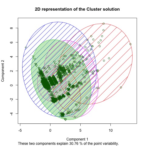 clustering of mindwave data
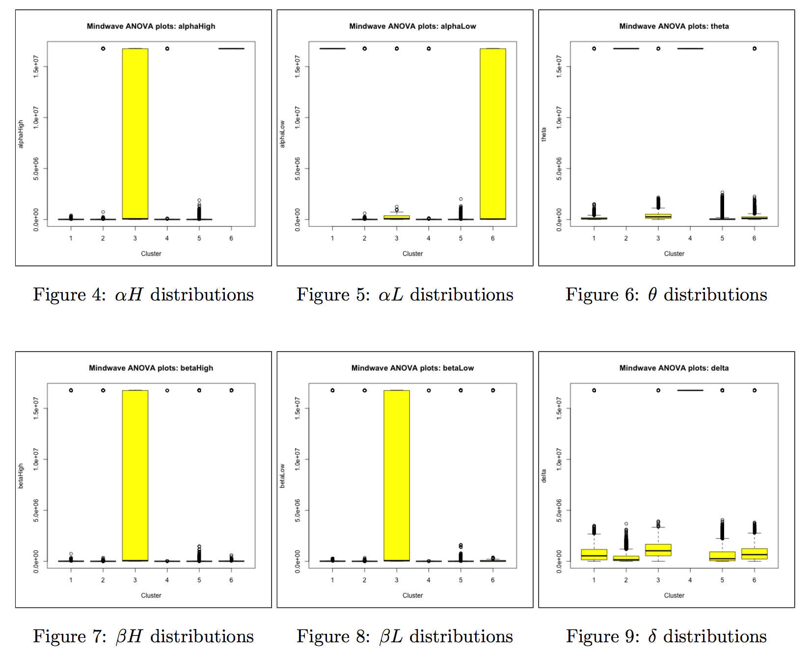
As the first two components of the Principal Component Analysis only captures 30.76% of the variance, the overall cluster distribution in space is more  -dimensional. We further conducted an ANOVA analysis for each data type (brainwaves, voltage and attention and meditation values) across all the clusters. Box plot visualizations of the first 6 key features are shown in Figures below. For the sake of simplicity, we have not shown and plots, even though both were statistically significant and were enriched for Cluster 3. We can qualitatively represent our clusters are as follows:-
- Cluster 1: very high
- Cluster 2: very high
- Cluster 3: very high
 , all ranges of , , , with a low median
 - Cluster 4: very high and
- Cluster 5: No values high – baseline
- Cluster 6: very high , all ranges of with a low median
Initially, we trained all our models using room  level as an indicator of occupant activity inside the room. We trained our models using data collected continuously over 5 days between October 10, 2015 to October 14, 2015. The trained models were tested on the data collected between October 19, 2015 to October 22, 2015. For our baseline, we predicted room temperature and relative humidity using only external weather data. For the oracle, we predicted room temperature using outside weather data, inside humidity and levels and inside humidity using outside weather data, levels and inside temperature. We used Root Mean Square Error between the predicted response variable and the actual response variable as our evaluation metric.
A comparison of the predicted temperature with the actual temperature for MLR has been plotted in Figures below. As suggested by the RMSE values and the plots, including information about activity levels of occupants inside the room improves the prediction accuracy. (RMSE value decreases as we move from the baseline to the model with and  as features). We also performed sequential variable selection on our and model to ensure that we were not overfitting with too many outside weather features. We followed a forward feature selection algorithm where we began with no features and kept adding features which improved the prediction accuracy on the validation set. From the feature selection results we inferred that all the outside weather features were important in prediction of inside temperature (and humidity) with outside temperature, wind speed, dewpoint, pressure and wind bearing being the top 5 outside weather features.
We also trained and tested AR and NAR models on the same dataset as MLR. For the AR models, we used a delay of 3 units for each input and a delay of 3 units for the output. For NAR, we used a delay of 4 units for each of the inputs and a delay of 2 units for the output. We used 16 hidden units in the hidden layer. These hyperparameters were chosen based on the model’s performance on a validation set. The trained models were used to make multiple step ahead predictions.
For AR, every 12 minutes of past inputs, actual past outputs and 12 minutes of future inputs were used to predict outputs 12 minutes into the future. The predicted outputs and corresponding RMSE values (using and as features) are shown in Figures below. Twelve step ahead prediction performance of AR looks promising. However, increasing the number of prediction steps beyond 12 minutes leads to degraded performance due to accumulation of prediction error.
For NAR, we performed a full closed loop prediction where only future inputs and predicted outputs are used as inputs for prediction over the entire prediction interval. We also preformed a one step ahead prediction where the actual values of the output were used to predict the next output value. The predicted outputs (for temperature) and corresponding RMSE values (using and as features) are shown in Figures below. The one step ahead performance of NAR is reasonable with a few outliers. However, the closed loop prediction is clearly erroneous due to accumulation of prediction error. Changing the hyperparameters and feature selection did not help in improving the closed loop performance of NAR. The closed loop performance on the training set was much better which indicates that the neural network is overfitting the data.
The next step was to use the occupant activity level labels derived from our occupant activity classification stage as indicators of activity inside the room. We had a total of  data points spanning across multiple data collection episodes. We could not train AR and NAR models on this dataset as the entire dataset as a whole was not continuous in time because the collection episodes spanned across several days and a single collection episode only had 60 points (corresponding to one hour). The RMSE values obtained for various feature combinations using MLR on this dataset are summarized in the table below:
Discussion
A crucial element of this project was the initial data collection effort, through which we attempted to create our own correlated database with occupant activity level, mental state and heart rate information as well as environmental conditions using a variety of sensors. No such database exists currently, that we are aware of, so we were limited to the data we created ourselves. Given that we had to discard the smart watch data, we were left with only 646 correlated occupant state – room state data points. This data proved not to be sufficient for some of the models and algorithms we initially had in mind, including a Markov Decision Process where we would control the environment conditions to encourage an improved occupant state, and AR and NAR models for room state prediction using occupant activity level labels.
Moreover, losing smart watch data, which contained information about the physiological state of the occupant proved more detrimental to the room state prediction part because the mindwave data only captures information about the mental state of the occupant which by itself is unlikely to cause a large impact on the room state. This explains the poor performance of MLR on the correlated occupant state – room state data.
Besides the limited number of data points, there are two other issues with the data: 1) we only have data corresponding to the three members of the team, and 2) they were collected while practicing similar activities. These issues impacted the diversity of the data and promoted a significant skew in the number of samples for the different occupant states, which in turn limited the learning capability of our algorithms.
Despite our issues with the dataset, we were still able to clearly distinguish 6 archetypes for occupant state. In essence, we established that cluster 5 represents the \textbf{Baseline State}, clusters 2 and 6 constitute the  , and clusters 3 and 4 constitute the
  . The rationale behind this choice, is that a higher value of
  is often associated with stress, anxiety and restlessness, whereas a higher value of represents an unconscious mind or a state of deep sleep, which is also undesirable when in meetings. It is at the
  border where the optimal range for visualization, mind programming and creativity develops, and these are enriched in clusters 2 and 6. Cluster 1 can be considered a \textbf{Suboptimal State} due to a higher value of .
We used iterated prediction scheme for multiple step ahead prediction in the AR model, where the predicted output is fed back as input to make multiple predictions into the future. This strategy is known to lead to suboptimal predictions because the model is trained only to predict one step ahead. Iterated prediction leads to accumulation of errors. The same holds true for NAR model as well.
In terms of the occupant state prediction, there are some encouraging results in terms of separating room conditions that lead to a Desirable State from those that lead to Undesirable states, although the significant skew in the data points clearly influenced the algorithms to better predict Desirable States than Undesirable States. This exploration must be continued with a larger, more varied dataset that can provide a better insight into what environmental conditions lead to Desirable mental states.
Conclusion
A better understanding of a building’s internal loads could have a significant impact on the way building performance is simulated and monitored. We set out to understand the impact that an occupant’s activity level can have on a room’s environmental conditions which would in turn affect the energy consumption of the building as the HVAC system reacts to the room’s changes. We also hypothesized that the insights gained from analyzing the occupant’s impact on the room could perhaps be used reversely – controlling the room’s environmental conditions in order to influence the occupant’s state.
The first step in our process was the generation of a correlated dataset tracking both the occupant’s and the room’s states. The occupant’s state was tracked using bio-physiological sensors through the use of smartwatches and Neurosky Mindwave. The smartwatches purpose was to obtain physiologial data while the Mindwave headsets gave us insight into the user’s mental state. Regrettably, the smartwatch data has to be discarded and the subsequent analysis were carried using mind state data and CO2 levels as a proxy for the activity level. Discarding the smartwatch data also significantly reduced the amount of correlated datapoints we could use for training and testing our algorithms. Given this, future work on this area will largely depend on the creation of a large, varied correlated dataset that includes several users -both their activity level and their mental state-, and longer data collection periods to obtain sufficient datapoints for adequately training the algorithms.
Despite the limited dataset, we had some encouraging results. First, we were able to cluster the mental states and classify each cluster as Desirable or Undesirable. Second, when using Multiple Linear Regression we found that including the activity level proxy improved our prediction of room state changes over our Baseline. On the other hand, we were limited to an iterated prediction scheme for multiple step ahead prediction and thus could not get adequate prediction several steps ahead. Another disadvantage was the inability to positively determine whether it would be possible to predict changes in occupant state through changes in the environmental conditions of the space they are in.
We believe our methodology is a solid step into better understanding the dynamics between occupants and spaces and how they impact each other. Replicating this process with a better dataset could provide invaluable information and can improve the quality of building performance simulation and monitoring.